Excel Automation – VBA to Help Make Surface-Plots
Imagine that you have a complicated excel spreadsheet that might have more than one variable and calculates a numerical output. And, you would like to make a surface plot of the result as the two variables change.
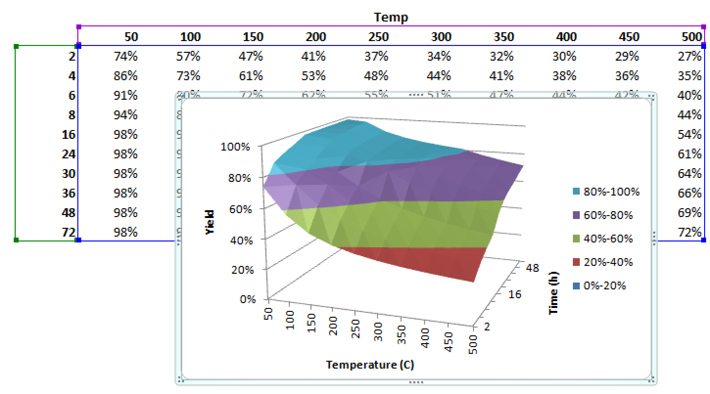
Surface plots are useful for displaying complicated data that tend to change a function of 2 or more parameters. For example, a product yield might depend on both temperature and reaction time. So, to make a surface plot showing this behavior, you would choose different times and temperatures and record the resulting yield. In this example, we picked 10 temperatures and 10 times. That is 100 scenarios that will need to be entered, calculated, recorded, and then plotted. – Do you really want to type a 100 different values and copy and paste each result to fill in the grid? What if you decide you picked the wrong range? Start over?
A faster method is to build a VBA Macro that can do the typing for you.
Here is what to do:
Start with your worksheet that does the calculations. Open it and have a single worksheet that accepts the inputs and gives the outputs.
Then out where you want the data to go… make a new workbook.
Next, define the range for analysis. Start by making an empty data grid. Your ranges for testing will go along the edges. In this example, time will vary from 2 to 72 hours and Temperature from 50 to 500. I have picked 10 times and temperatures and entered the values that I want to test here on the worksheet. The calculated result will go in the cell that crosses the row and column.

Open Visual Basic Editor (in Excel’s Developer Tab
Create a new module (Insert > Module) and put it in your personal workbook for future use.
There is an editor window for your module. It looks like an empty text file. You can open modules by double clicking on them. New modules will be blank…
Start by defining a subroutine called TestProgram(). The command Sub indicates it is subroutine, followed by its name, and () is where you would define pass through variables from another macro.
Type:
Sub TestProgram()
Press enter.
End Sub should appear at the bottom of the editor to automatically close off the subroutine.
Press enter again to leave some space.
Now we will define a For loop for the rows and columns. A For loop defines a variable and sets it equal to a starting number. For n = 1 to 10 step 1 will create a variable n and set it equal to 1. Any commands between For n = 1 to 10 step 1 and Next n will be executed. When the commands have run, a Next n statement will tell n to increment by the value defined by step and repeat the process. Here, step 1 means n goes from n to n+1 and then the commands execute again. The process keeps going until n = 10. These loops can be nested and the inner most loop finishes before the outermost loop.
We use two For loops to move along the rows and columns of the data grid. The row loop is nested in the column loop. So, it will fix a column and move down the column by incrementing the rows by 1. Them move to the next column. I entered 10 different times and temperatures that I wanted to test in the empty data grid, so we set the upper limit at 10.
Type:
For n = 1 to 10 step 1
For r = 1 to 10 step 1
You needed to have an open workbook to get the variables and store the results. We need to make sure that file is active first. In this example, “Price Comparison.xlsx” is the name of my workbook where the results will be saved.
Type:
Windows(“Price Comparison.xlsx”).Activate
Now, define two internal variables to store the values you want to test. The variable (HydroT and SL) will be set to the values you entered in the empty grid. In this example, the Times are in a column, so the row will increment downward with each iteration. The Cells() command tells VBA to go to the currently active sheet and look for that cell. Here, we are going to use Cells(row + offset from the top, column the values are in). We include an offset to account for the distance from the edges of the worksheet. So, the first Time we want to test is 6 rows down from the top and three columns in from the left edge. So, that is 5 empty cells + r, and r starts at 1. The temperature values are in row 5 and start in column D, or 3 empty columns + n over from the left side.
Remember that r is the row and n is the column variable the will change during the For loop. And will increment along the rows and columns were you put the conditions you wanted to test.
Type:
HydroT = Cells(5 + r, 3).Value
SL = Cells(5, 3 + n).Value
Now, we switch to the workbook that does the calculations.
Type:
Windows(“RL-SingleProduct-V7(60pct).xlsm”).Activate
In this example, my calculations are done is RL-SingeProduct-V7(60pct).xlsm workbook. You will replace this text with the name of your workbook.
Now, in the calculation workbook. I assume you only have one worksheet active… You need put the variables into the worksheet’s appropriate cells. For this, you can either use the Cells(row,column) function or the less direct Range() command. The Range() command calls out name of the cell, which can also be a named label. In my example cell C23 is the time entry cell and G25 is the temperature entry cell. So, Range(“C23”).Select activates the cell and ActiveCell.FormulaR1C1 = HydroT passes the value of the HydroT into the cell. We could also use Cells(23,3).Value = HydroT to put the value into the cell. My calculating spreadsheet uses iteration on selection. So, I have included an additional Range(“G25”).Select to force the sheet to re-iterate.
Type:
Range(“C23”).Select
ActiveCell.FormulaR1C1 = HydroT
Range(“G25”).Select
ActiveCell.FormulaR1C1 = SL
Range(“G25”).Select
Now, we need to get the results back into the macro and put them into the starting workbook. For my workbook, the result comes out in cell H2. So, we collect the value and put it into the variable temp for safe keeping. I am using the Range() command, Cells(2,9).Value would work as well. The Rage() would let me call out a named cell later for another project. That would also let me move the results to a any location in the file and Excel will follow the name’s pointed location and not an absolute cell reference. This a good option if you don’t have everything on a single worksheet.
Type:
temp = Range(“H2”).Value
The value is now stored in temp. Next, go back to the workbook that will store the results.
Type:
Windows(“Price Comparison.xlsx”).Activate
Excel needs to put the values into the cell in the grid. The calculated answers are the intersection of the two variables. In my example, that starts at row 6 and column 4. We offset the row by 6 to move down 6 lines. So, we take r and add 6 to it. The column starts in column D, that is 4 columns from the left. So, take the column variable n and add 3 to move over 3 spots. Remember that r and n start at 1 and count to 10. Set the value of the cell to the result stored in temp.
Type:
Cells(5 + r, 3 + n) = temp
We need to increment the r and n to do the next iteration. We nested the rows in the columns. So, we need to increment the rows first. After the macro goes from row 1 to row 10, then it will go to the next column and do rows 1 to 10 again. The order of Next r and Next n matter.
Type:
Next r
Next n
Your macro should end with End Sub to tell it that your subroutine is done.

Save everything!
Now with the calculating workbook open and the input/output worksheet selected, and the results workbook open and selected to the worksheet with the variables grid, run the macro. You can goto the VBA editor window, click in the macro code area and then click the green Play Button, use the menu to choose Run > Run Sub/User Form, or use the Developer ribbon and click on Macros to choose the macro you just made. The macro will work and report the data back into the grid.

Now you can create your 3D surface plot by selecting the data block and inserting a surface plot.  Add some labels, analysis and …
Done!
Hope this helps save you time.
